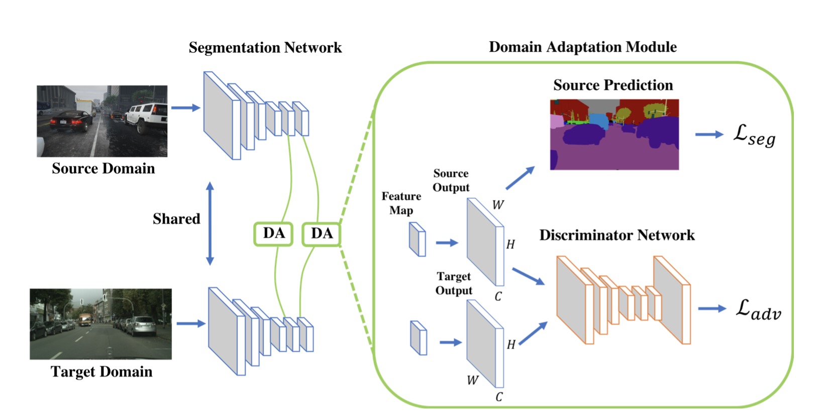
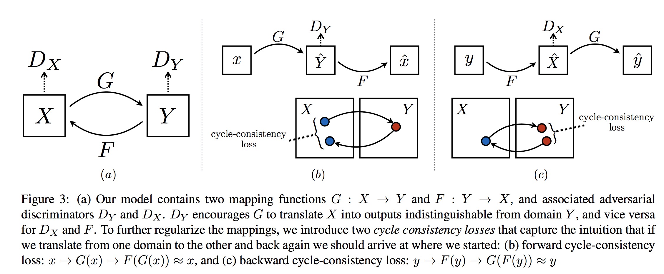
最近在看domain adaptation的代码,需要学习pytorch,然后参考莫烦python的代码,自己整理一遍:
用 Numpy 还是 Torch
Torch 自称为神经网络界的 Numpy, 因为他能将 torch 产生的 tensor 放在 GPU 中加速运算 (前提是你有合适的 GPU), 就像 Numpy 会把 array 放在 CPU 中加速运算. 所以神经网络的话, 当然是用 Torch 的 tensor 形式数据最好咯. 就像 Tensorflow 当中的 tensor 一样.
当然, 我们对 Numpy 还是爱不释手的, 因为我们太习惯 numpy 的形式了. 不过 torch 看出来我们的喜爱, 他把 torch 做的和 numpy 能很好的兼容. 比如这样就能自由地转换 numpy array 和 torch tensor 了:
1 | import torch |
Torch 中的数学运算
简单运算
其实 torch 中 tensor 的运算和 numpy array 的如出一辙, 我们就以对比的形式来看. 如果想了解 torch 中其它更多有用的运算符,API就是你要去的地方.
1 | # abs 绝对值的计算 |
矩阵的运算
除了简单的计算, 矩阵运算才是神经网络中最重要的部分. 所以我们展示下矩阵的乘法. 注意一下包含了一个 numpy 中可行, 但是 torch 中不可行的方式.1
2
3
4
5
6
7
8
9
10
11
12
13
14
15
16
17# matrix multiplication 矩阵点乘
data = [[1,2], [3,4]]
tensor = torch.FloatTensor(data) # 转换成32位浮点 tensor
# correct method
print(
'\nmatrix multiplication (matmul)',
'\nnumpy: ', np.matmul(data, data), # [[7, 10], [15, 22]]
'\ntorch: ', torch.mm(tensor, tensor) # [[7, 10], [15, 22]]
)
# !!!! 下面是错误的方法 !!!!
data = np.array(data)
print(
'\nmatrix multiplication (dot)',
'\nnumpy: ', data.dot(data), # [[7, 10], [15, 22]] 在numpy 中可行
'\ntorch: ', tensor.dot(tensor) # torch 会转换成 [1,2,3,4].dot([1,2,3,4) = 30.0
)
新版本中(>=0.3.0), 关于 tensor.dot() 有了新的改变, 它只能针对于一维的数组. 所以上面的有所改变.1
2
3
4tensor.dot(tensor) # torch 会转换成 [1,2,3,4].dot([1,2,3,4) = 30.0
# 变为
torch.dot(tensor.dot(tensor)
Variable
什么是Variable
这个感觉和tensorflow里面的一样,就是存有变化的数值的地方,然后这个变化的值就是tensor。然后,这里Variable可能有点像tensorflow里面的placeholder吧
1 | import torch |
Variable 计算,梯度
我们再对比一下 tensor 的计算和 variable 的计算.1
2
3
4t_out = torch.mean(tensor*tensor) # x^2
v_out = torch.mean(variable*variable) # x^2
print(t_out)
print(v_out) # 7.5
这里我们应该也看不出Variable和一般tensor的不同,和tensorflow类似,Variable参与计算时,也是在打一个computational graph (原来是将所有的计算步骤 (节点) 都连接起来, 最后进行误差反向传递的时候, 一次性将所有 variable 里面的修改幅度 (梯度) 都计算出来, 而 tensor 就没有这个能力啦,毕竟,tensor 只是一个值而已。)
v_out = torch.mean(variable*variable) 就是在计算图中添加的一个计算步骤, 计算误差反向传递的时候有他一份功劳, 我们就来举个例子:
1 | v_out.backward() # 模拟 v_out 的误差反向传递 |
获取 Variable 里面的数据
直接print(variable)只会输出 Variable 形式的数据, 在很多时候是用不了的(比如想要用 plt 画图), 所以我们要转换一下, 将它变成 tensor 形式.1
2
3
4
5
6
7
8
9
10
11
12
13
14
15
16
17
18
19
20print(variable) # Variable 形式
"""
Variable containing:
1
2
3
4
[torch.FloatTensor of size 2x2]
"""
print(variable.data) # tensor 形式
"""
1
2
3
4
[torch.FloatTensor of size 2x2]
"""
print(variable.data.numpy()) # numpy 形式
"""
[[ 1. 2.]
[ 3. 4.]]
"""
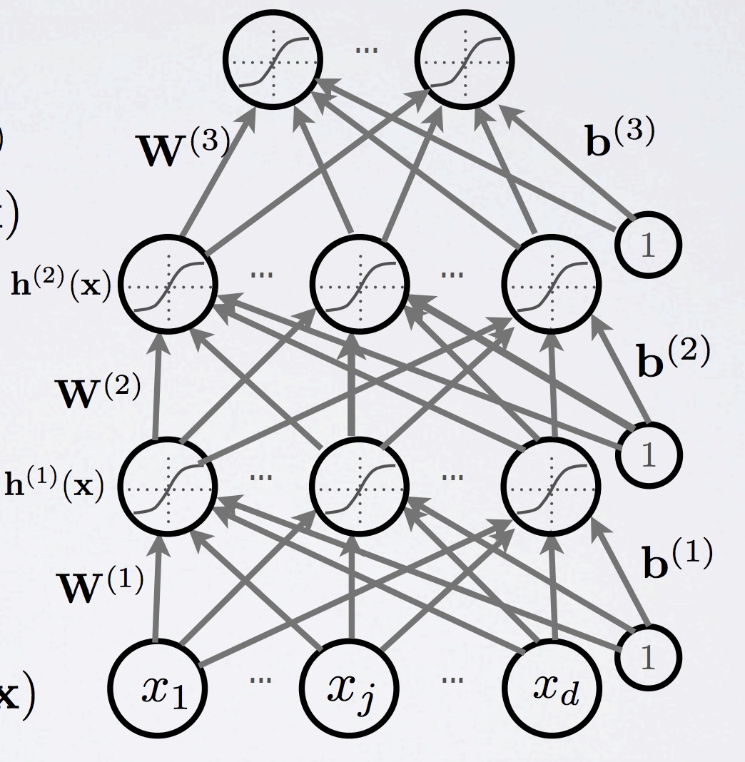
Activation
什么是 Activation
为什么需要非线性的函数?
- 线性的话,你多少层都一样
- 非线性的话,可以拟合不同的函数
Torch 中的激励函数
Torch 中的激励函数有很多, 不过我们平时要用到的就这几个. relu, sigmoid, tanh, softplus. 那我们就看看他们各自长什么样啦.
1 | import torch |
接着就是做生成不同的激励函数数据:1
2
3
4
5
6
7
8x_np = x.data.numpy() # 换成 numpy array, 出图时用
# 几种常用的 激励函数
y_relu = F.relu(x).data.numpy()
y_sigmoid = F.sigmoid(x).data.numpy()
y_tanh = F.tanh(x).data.numpy()
y_softplus = F.softplus(x).data.numpy()
# y_softmax = F.softmax(x) softmax 比较特殊, 不能直接显示, 不过他是关于概率的, 用于分类
接着我们开始画图, 画图的代码也在下面: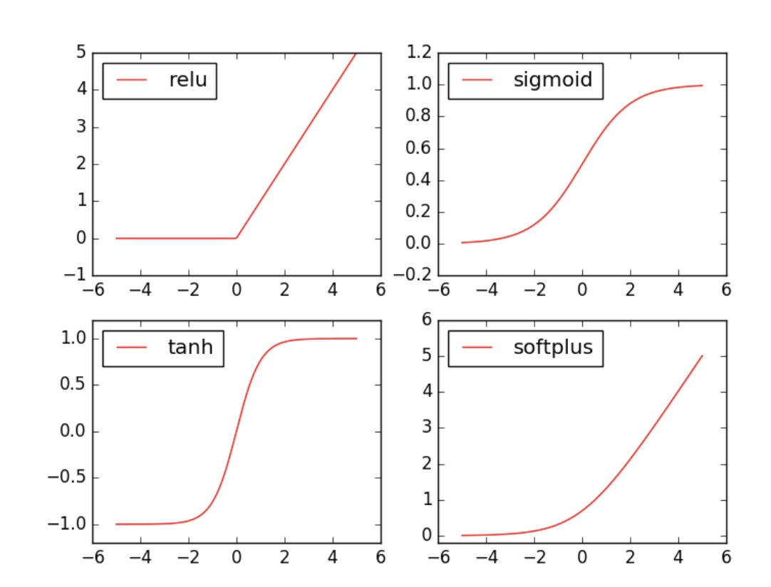
1 | import matplotlib.pyplot as plt # python 的可视化模块, 我有教程 (https://morvanzhou.github.io/tutorials/data-manipulation/plt/) |