311. Sparse Matrix Multiplication

Given two sparse matrices A and B, return the result of AB.

You may assume that A’s column number is equal to B’s row number.

Example:

1
2
3
4
5
6
7
8
9
10
11
12
13
14
15
16
17
18

Input:

A = [
  [ 1, 0, 0],
  [-1, 0, 3]
]

B = [
  [ 7, 0, 0 ],
  [ 0, 0, 0 ],
  [ 0, 0, 1 ]
]

Output:

     |  1 0 0 |   | 7 0 0 |   |  7 0 0 |
AB = | -1 0 3 | x | 0 0 0 | = | -7 0 3 |
                  | 0 0 1 |

Idea

normally,

1
2
3
4

for i in range(n):
    for j in range(m):
        for k in range(k):
            C[i][j] = A[i][k] * B[k][i]

In fact, this is same as

1
2
3
4

for i in range(n):
    for k in range(k):
        for j in range(m):
            C[i][j] = A[i][k] * B[k][i]

In this form, each A[i][k] may multiply a row of B, when a is 0, we can ignore it. What’s more, we can record the indexes of non-zero elements in a row of B, which also fasten the computation.

Code

1
2
3
4
5
6
7
8
9
10
11
12
13
14
15
16
17
18
19
20
21
22
23
24
25
26

class Solution(object):
    def multiply(self, A, B):
        """
        :type A: List[List[int]]
        :type B: List[List[int]]
        :rtype: List[List[int]]
        """
        n, p, m = len(A), len(A[0]), len(B[0])
        C = [[0] * m for _ in range(n)]
        
        cols = []
        for k in range(p):
            tmp = []
            for j in range(m):
                if B[k][j] != 0:
                    tmp.append(j)
            cols.append(tmp)
        
        for i in range(n):
            for k in range(p):
                if A[i][k] == 0:
                    continue
                for j in cols[k]:
                    C[i][j] += A[i][k] * B[k][j]
                    
        return C

91. Decode Ways

A message containing letters from A-Z is being encoded to numbers using the following mapping:

‘A’ -> 1
‘B’ -> 2
…
‘Z’ -> 26
Given a non-empty string containing only digits, determine the total number of ways to decode it.

Example 1:

Input: “12”
Output: 2
Explanation: It could be decoded as “AB” (1 2) or “L” (12).
Example 2:

Input: “226”
Output: 3
Explanation: It could be decoded as “BZ” (2 26), “VF” (22 6), or “BBF” (2 2 6).

Idea

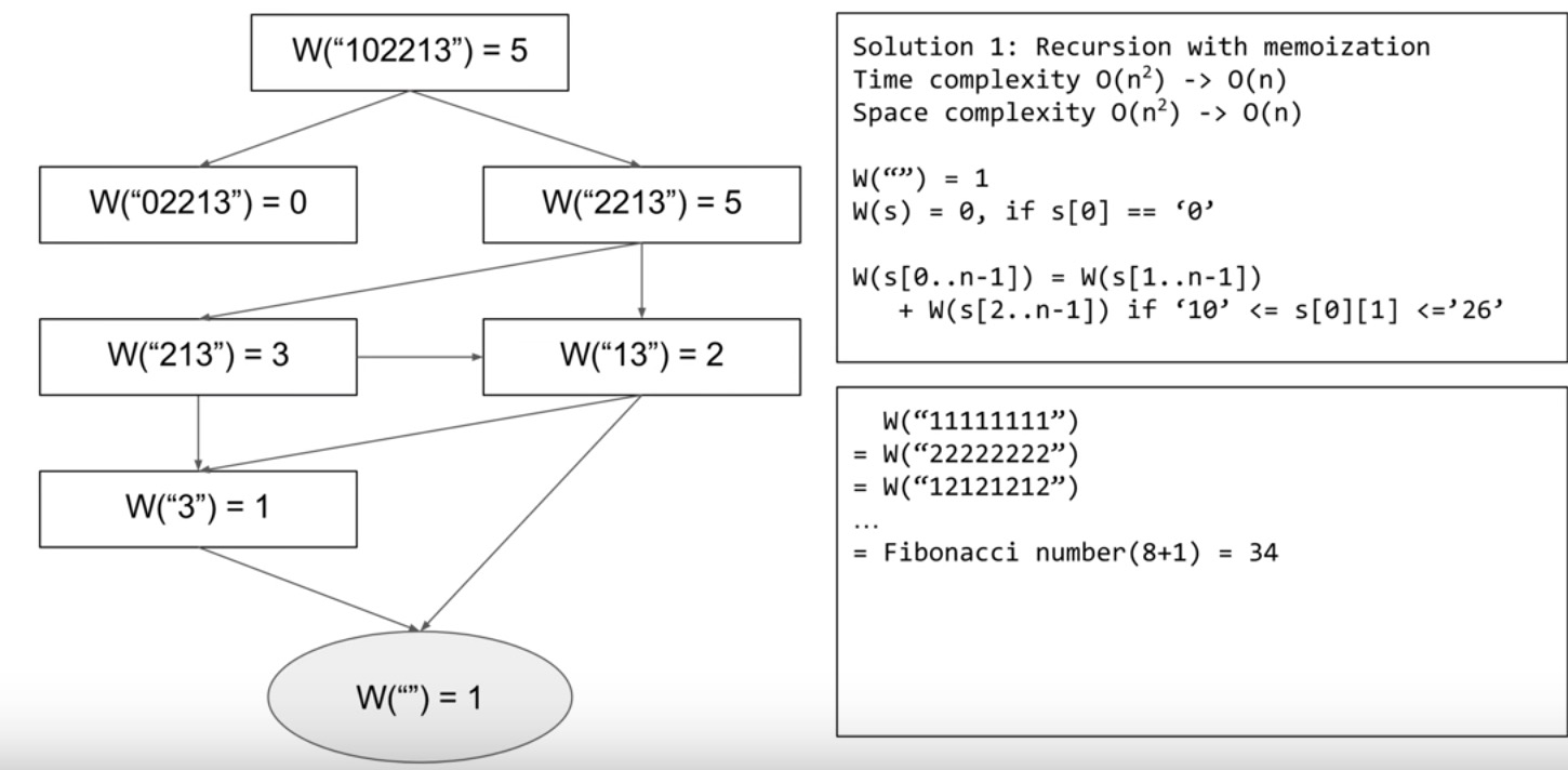
from 花花酱

Code

1
2
3
4
5
6
7
8
9
10
11
12
13
14
15
16
17
18
19
20
21
22
23
24
25
26
27

class Solution(object):
    def numDecodings(self, s):
        """
        :type s: str
        :rtype: int
        """
        if not s:
            return 0
        self.cache = {"":1}
        return self.dp(s)

    def dp(self, s):
        # base case
        if s in self.cache:
            return self.cache[s]
        if s[0] == '0':
            return 0
        if len(s) == 1:
            return 1
        
        w = self.dp(s[1:])
        if int(s[:2]) <= 26:
            w += self.dp(s[2:])
        
        # cache 
        self.cache[s] = w
        return w

48. Rotate Image

You are given an n x n 2D matrix representing an image.

Rotate the image by 90 degrees (clockwise).

Note:

You have to rotate the image in-place, which means you have to modify the input 2D matrix directly. DO NOT allocate another 2D matrix and do the rotation.

Example 1:

Given input matrix =
[
[1,2,3],
[4,5,6],
[7,8,9]
],

rotate the input matrix in-place such that it becomes:
[
[7,4,1],
[8,5,2],
[9,6,3]
]

Idea

tranpose firtly and mirror translate second.

Code

1
2
3
4
5
6
7
8
9
10
11
12
13
14
15
16
17
18
19
20
21
22
23
24

class Solution:
    """
    @param matrix: a lists of integers
    @return: nothing
    """
    def rotate(self, matrix):
        # write your code here
        if matrix == None or len(matrix) == 0:
            return None
        matrix = self.transpose(matrix)
        matrix = self.mirror(matrix)
        return matrix

    def mirror(self, matrix):
        for i in range(len(matrix)):
            matrix[i].reverse()        
        return matrix
        
    def transpose(self, matrix):
        n = len(matrix)
        for i in range(n):
            for j in range(i, n):
                matrix[i][j], matrix[j][i] = matrix[j][i], matrix[i][j]
        return matrix

Python

1
2
3
4

# list reverse
matrix[i].reverse()
# exchange
matrix[i][j], matrix[j][i] = matrix[j][i], matrix[i][j]

43. Multiply Strings

Given two non-negative integers num1 and num2 represented as strings, return the product of num1 and num2, also represented as a string.

Example 1:

Input: num1 = “2”, num2 = “3”
Output: “6”
Example 2:

Input: num1 = “123”, num2 = “456”
Output: “56088”
Note:

The length of both num1 and num2 is < 110.
Both num1 and num2 contain only digits 0-9.
Both num1 and num2 do not contain any leading zero, except the number 0 itself.
You must not use any built-in BigInteger library or convert the inputs to integer directly.

Idea

Simply thinking, decompose the multiplication into multiply num1 with each bit of num2 and add them together.

Code

1
2
3
4
5
6
7
8
9
10
11
12
13
14
15
16
17
18
19
20
21
22
23
24
25
26
27
28
29
30
31
32
33
34
35
36
37
38
39
40
41
42
43
44
45
46
47
48
49
50
51
52
53
54
55
56
57
58
59
60
61
62

class Solution:
    """
    @param num1: a non-negative integers
    @param num2: a non-negative integers
    @return: return product of num1 and num2
    """
    def __init__(self):
        self.d = {str(i): i for i in range(0, 10)}
        self.s = {i: str(i) for i in range(0, 10)}
	
    def multiply(self, num1, num2):
        # num1 is smaller number
        if num1 == '0' or num2 == '0':
            return '0'
        
        total_sum = "0"
        for i, figure in enumerate(num1[::-1]):
            term = self.single_multiply(num2, figure) + "0" * i
            total_sum = self.add(term, total_sum)
        return total_sum
            
    def single_multiply(self, num, bit):
        idx = len(num) - 1
        b = self.d[bit]
        carry = 0
        cur = 0
        res = ''
        while idx >= 0:
            n1 = self.d[num[idx]]
            cur = (n1 * b + carry) % 10
            carry = (n1 * b + carry) / 10
            res = self.s[cur] + res
            idx -= 1
        
        if carry > 0:
            res = self.s[carry] + res
        return res
    
    def add(self, num1, num2):
        if not num1:
            num1 = '0'
        if not num2:
            num2 = '0'

        idx1 = len(num1) - 1
        idx2 = len(num2) - 1 
        
        res = ''
        cur = 0
        carry = 0
        while idx1 >= 0 or idx2 >= 0:
            n1 = self.d[num1[idx1]] if idx1 >= 0 else 0
            n2 = self.d[num2[idx2]] if idx2 >= 0 else 0
            cur = (n1 + n2 + carry) % 10
            carry = (n1 + n2 + carry) / 10
            res = self.s[cur] + res
            idx1 -= 1
            idx2 -= 1
        if carry == 1:
            res = '1' + res

        return res

Python

1
2
3
4
5

a = [1, 2, 3, 4]
print(a[len(a) - 1::-1])
print(a[::-1]) # omission
[4, 3, 2, 1]
[4, 3, 2, 1]

Object Detection

To what extent do [Krizhevsky et. al’s results] generalize to object detection?

Object detection is the task of finding the different objects in an image and classifying them

mAP (mean average precision)

This blog explain the mAP clearly.

RCNN

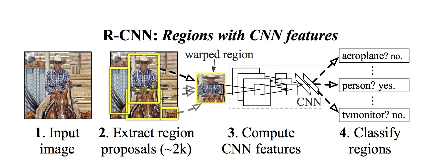
The goal of R-CNN is to take in an image, and correctly identify where the main objects (via a bounding box) in the image.

Inputs: Image
Outputs: Bounding boxes + labels for each object in the image.

region proposals:

At a high level, Selective Search (shown in the image above) looks at the image through windows of different sizes, and for each size tries to group together adjacent pixels by texture, color, or intensity to identify objects.

feature extraction:

They extract a 4096-dimensional feature vector from each region proposal using the Caffe implementation of the CNN described by Krizhevsky et al.. Features are computed by forward propagating a mean-subtracted 227 × 227 RGB image through five convolutional layers and two fully connected layers.

Since the sizes of boxes from region proposals varies, they need firstly warp image data in that region into a form that is compatible with the CNN (its architecture requires inputs of a fixed 227 × 227 pixel size)

training:

Supervised pre-training

They discriminatively pre-trained the CNN on a large auxiliary dataset (ILSVRC2012 classification) using image-level annotations only (bounding-box labels are not available for this data).

Domain-specific fine-tuning.

To adapt our CNN to the new task (detection) and the new domain (warped proposal windows), we continue stochastic gradient descent (SGD) training of the CNN parameters using only warped region proposals with a bias ratio mini-batch amoung negative and positive samples which are assigned according to the IoU larger than 0.5 or not.

Object category classifiers.

Similar to the step above, given threshold split the data set into negative and positve samples for classification in SVM.

Summary

• Generate a set of proposals for bounding boxes.
• Run the images in the bounding boxes through a pre-trained AlexNet and finally an SVM to see what object the image in the box is.
• Run the box through a linear regression model to output tighter coordinates for the box once the object has been classified.

Problems:

1. Training is a multi-stage pipeline. R-CNN first fine-tunes a ConvNet on object proposals using log loss. Then, it fits SVMs to ConvNet features. These SVMs act as object detectors, replacing the softmax classifier learnt by fine-tuning. In the third training stage, bounding-box regressors are learned.
2. Training is expensive in space and time. For SVM and bounding-box regressor training, features are extracted from each object proposal in each image and written to disk. With very deep networks, such as VGG16, this process takes 2.5 GPU-days for the 5k images of the VOC07 trainval set. These features require hundreds of gigabytes of storage.
3. Object detection is slow. At test-time, features are extracted from each object proposal in each test image. Detection with VGG16 takes 47s / image (on a GPU).

Fast-RCNN

Architecture

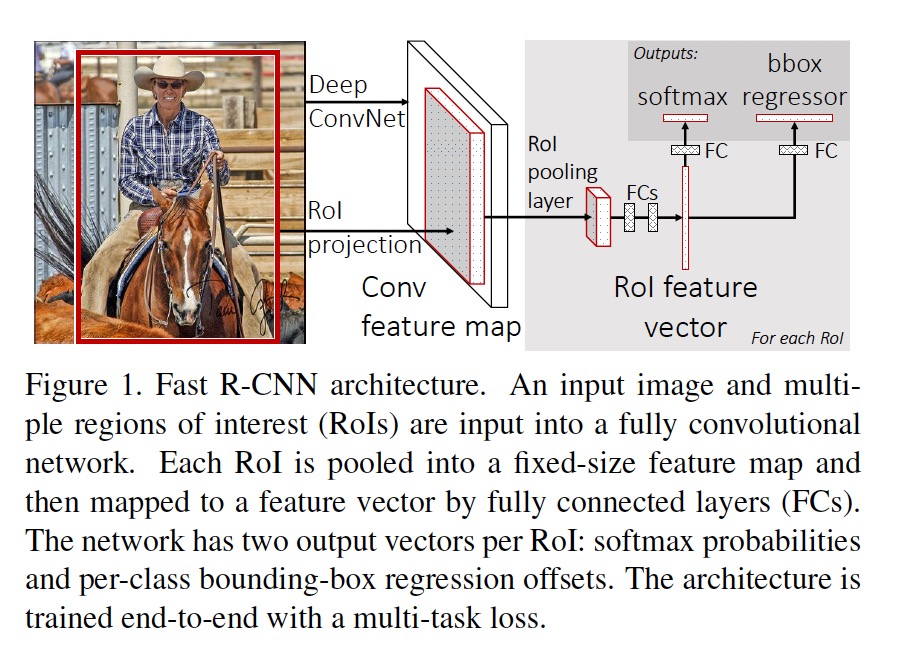
The input images as well as a set of region proposals are forwarded through a conv network and projected to a feature map. The feature map for each projected region proposal is processed via the RoI pooling layer and FCs into a fix-size RoI feature vector. Each feature vector is then fed into a sequence of fully connected layers (FC) that finally branch into two sibling output layers: one that produces softmax probability estimates over K object classes plus a catch-all “background” class and another layer that outputs four real-valued numbers for each of the K object classes. Each set of 4 values encodes refined bounding-box positions for one of the K classes.

RoI (Region of Interest) pooling layer

Similary to the warping in RCNN to process the region proposal into a fix-size input of fine-tune netowrk, the RoI max pooling works by dividing the h  w RoI window into an H  W grid of sub-windows of approximate size h=H  w=W and then max-pooling the values in each sub-window into the corresponding output grid cell.

Training

• step1: pre-trained:
  Amoung three pre-trained network from ImageNet the last max pooling layer is replaced by a RoI pooling layer that is configured by setting H and W to be compatible with the net’s first fully connected layer and last fully connected layer and softmax are replaced with the two sibling layers.

• step2: fine-tune:

  • summary:
    • mini-batch:
      In Fast RCNN training, stochastic gradient descent (SGD) minibatches are sampled hierarchically, first by sampling N images and then by sampling R=N RoIs from each image.
    • end-to-end:
      Fast R-CNN uses a streamlined training process with one fine-tuning stage that jointly optimizes a softmax classifier and bounding-box regressors, rather than training a softmax classifier, SVMs, and regressors in three separate stages.
  • loss: multi-task loss:
    $L(p, u, t^u, v) = L_{cls}(p, u) + \lambda_{[u > 0]}L_{loc}(t^u, v)$
    Each training RoI is labeled with a ground-truth class u and a ground-truth bounding-box regression target v. We use a multi-task loss L on each labeled RoI to jointly train for classification and bounding-box regression:
    • $L_{cls}(p(x), u) = - log p_u$
      classification loss is log loss for true class u
    • $L_{loc}(t^u, v) = \sum_{i \in {x, y, w, h}} smooth_{L_1} (t_i^u - v)$
      is a robust L1 loss that is less sensitive to outliers than the L2 loss used in R-CNN and SPPnet. When the regression targets are unbounded, training with L2 loss can require careful tuning of learning rates in order to prevent exploding gradients.

  • mini-batch:

    • sharing weights:
      each SGD mini-batch is constructed from N = 2 images, chosen uniformly at random (as is common practice, we actually iterate over permutations of the dataset). We use mini-batches of size R = 128, sampling 64 RoIs from each image.
    • ratio: Similar to the ratio mini-batch in RCNN, 25 % RoIs IoU at least 0.5 are as positive images (with ground truth labels), [0.1, 0.5) are as back-ground.

Pre-knowledge review

DQN

• loss function:
  $I = (r + \gamma max_{a’} Q(s’, a’, w_{-} - Q(s, a, w)))^2$
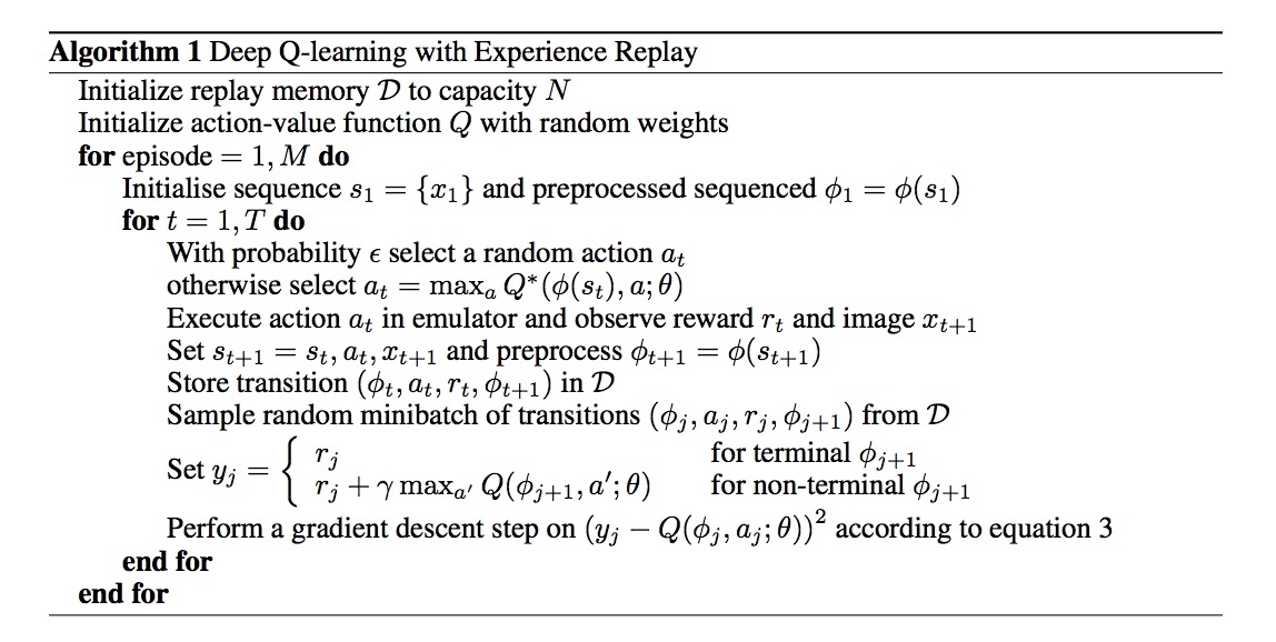
  Deep Q Learning implement the q-network to approximate Q function in place of a huge state table. In the training stage, our target data may gain from Q-network with old weight to update the new weight, which is very similar to supervised learning, while DQN is not.

• algorithm
  

A2C

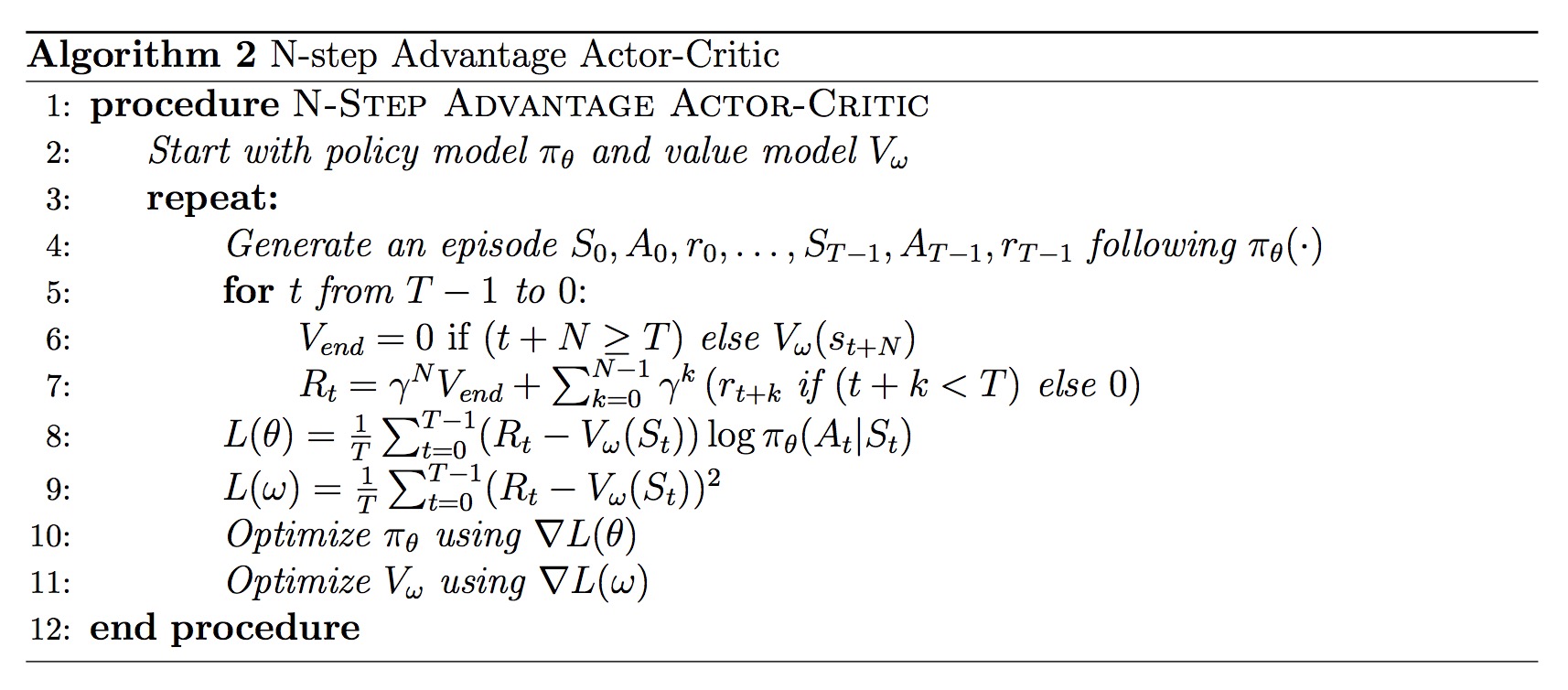
• loss
  

• algorithm
  

DDPG

Naive analysis may start from the decomposition three phrases: deep + Deterministic + Policy Gradient (from )

Deep

In fact, in DQN, we have two weights, or two network, one to predict the future Q value with old weight, and one to be updated. Also, we may perform the memory replay.

Deterministic

Deterministic Action taken rather than sample from a distribution.

Policy Gradient

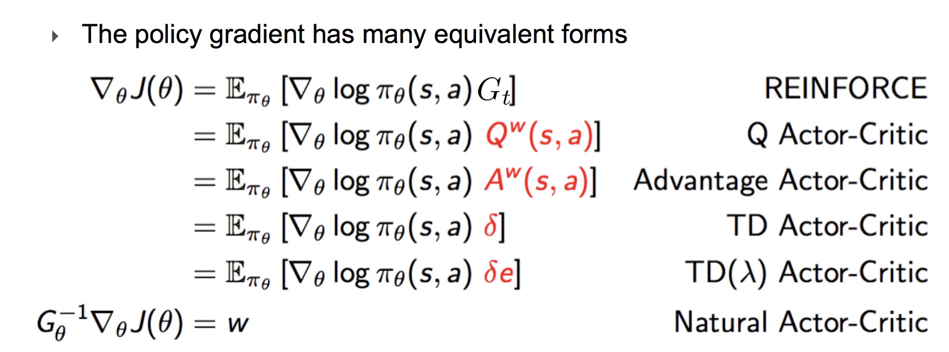
• actor
  Policy Gradient

• critic
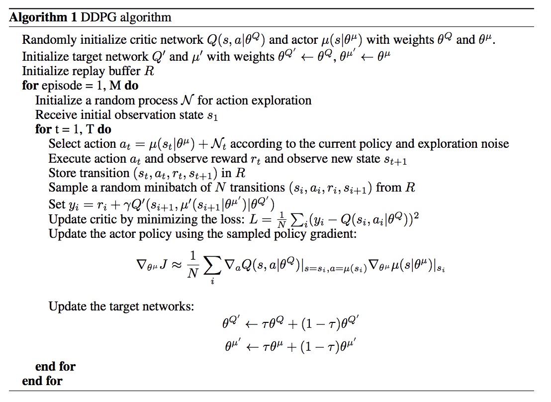
  Value-based

• algorithm
  

RNN

Motivation

If our inputs and outputs are sequences, the structure of the DNN may vary due to different length of inputs and outputs. Also, traditional DNN may not abstract the temporary feature from the sequences. So, a new network which include information flow from previous states and share the weight in each single local structure may achieve our requirements.

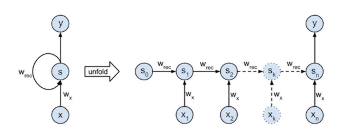
Structure

BPTT

Implementation

Dataset Define

1
2
3
4
5
6
7
8
9

# Create dataset
nb_of_samples = 20
sequence_len = 10
# Create the sequences
X = np.zeros((nb_of_samples, sequence_len))
for row_idx in range(nb_of_samples):
    X[row_idx,:] = np.around(np.random.rand(sequence_len)).astype(int)
# Create the targets for each sequence
t = np.sum(X, axis=1)

forward

1
2
3
4
5
6
7
8
9
10
11
12
13
14
15
16
17
18
19
20
21
22
23
24
25
26
27
28
29
30

# Define the forward step functions
def update_state(xk, sk, wx, wRec):
    """
    Compute state k from the previous state (sk) and current input (xk),
    by use of the input weights (wx) and recursive weights (wRec).
    """
    return xk * wx + sk * wRec

def forward_states(X, wx, wRec):
    """
    Unfold the network and compute all state activations given the input X,
    and input weights (wx) and recursive weights (wRec).
    Return the state activations in a matrix, the last column S[:,-1] contains the
    final activations.
    """
    # Initialise the matrix that holds all states for all input sequences.
    # The initial state s0 is set to 0.
    S = np.zeros((X.shape[0], X.shape[1]+1))
    # Use the recurrence relation defined by update_state to update the 
    #  states trough time.
    for k in range(0, X.shape[1]):
        # S[k] = S[k-1] * wRec + X[k] * wx
        S[:,k+1] = update_state(X[:,k], S[:,k], wx, wRec)
    return S

def cost(y, t): 
    """
    Return the MSE between the targets t and the outputs y.
    """
    return ((t - y)**2).sum() / nb_of_samples

back-progapation

1
2
3
4
5
6
7
8
9
10
11
12
13
14
15
16
17
18
19
20
21
22
23
24
25

def output_gradient(y, t):
    """
    Compute the gradient of the MSE cost function with respect to the output y.
    """
    return 2.0 * (y - t) / nb_of_samples

def backward_gradient(X, S, grad_out, wRec):
    """
    Backpropagate the gradient computed at the output (grad_out) through the network.
    Accumulate the parameter gradients for wX and wRec by for each layer by addition.
    Return the parameter gradients as a tuple, and the gradients at the output of each layer.
    """
    # Initialise the array that stores the gradients of the cost with respect to the states.
    grad_over_time = np.zeros((X.shape[0], X.shape[1]+1))
    grad_over_time[:,-1] = grad_out
    # Set the gradient accumulations to 0
    wx_grad = 0
    wRec_grad = 0
    for k in range(X.shape[1], 0, -1):
        # Compute the parameter gradients and accumulate the results.
        wx_grad += np.sum(grad_over_time[:,k] * X[:,k-1])
        wRec_grad += np.sum(grad_over_time[:,k] * S[:,k-1])
        # Compute the gradient at the output of the previous layer
        grad_over_time[:,k-1] = grad_over_time[:,k] * wRec
    return (wx_grad, wRec_grad), grad_over_time

Problem

If you regard each layer in time flow as a layer in DNN, then the RNN somehow is a kind of DNN, while there’s an input in each layer. The BP of RNN (BPTT) is very similar to BP in DNN. Thus, if the length of RNN is large enough, then BPTT may suffer from gradient explosion and gradient vanishing.

Solution

• gradient explosion:
  The clipping may solve the problem of explosion

• gradient vanishing:
  We may need modification of the traditional RNN structure. Thus, GRU and LSTM came into being.

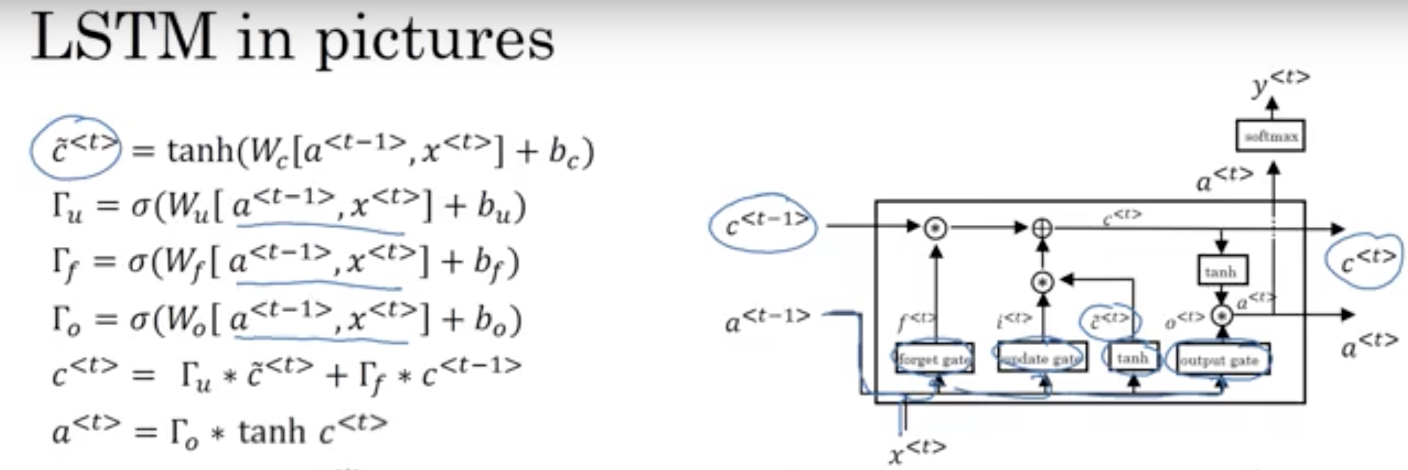
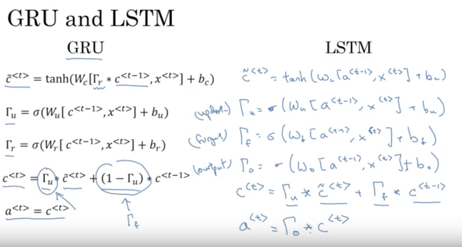
LSTM

The chain rule results in vanishing, thus, if we change this structue into combination of sum terms.

The cell state in LSTM is linear combination of current state and previous state, which avoid the gradient vanishing.

GRU

The GRU simplifies the output and remove forget gate in LSTM.