RNN

RNN

Motivation

If our inputs and outputs are sequences, the structure of the DNN may vary due to different length of inputs and outputs. Also, traditional DNN may not abstract the temporary feature from the sequences. So, a new network which include information flow from previous states and share the weight in each single local structure may achieve our requirements.
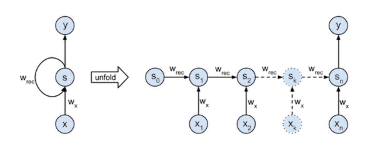
Structure

BPTT

Implementation

Dataset Define

1
2
3
4
5
6
7
8
9
# Create dataset
nb_of_samples = 20
sequence_len = 10
# Create the sequences
X = np.zeros((nb_of_samples, sequence_len))
for row_idx in range(nb_of_samples):
X[row_idx,:] = np.around(np.random.rand(sequence_len)).astype(int)
# Create the targets for each sequence
t = np.sum(X, axis=1)

forward

1
2
3
4
5
6
7
8
9
10
11
12
13
14
15
16
17
18
19
20
21
22
23
24
25
26
27
28
29
30
# Define the forward step functions
def update_state(xk, sk, wx, wRec):
"""
Compute state k from the previous state (sk) and current input (xk),
by use of the input weights (wx) and recursive weights (wRec).
"""
return xk * wx + sk * wRec

def forward_states(X, wx, wRec):
"""
Unfold the network and compute all state activations given the input X,
and input weights (wx) and recursive weights (wRec).
Return the state activations in a matrix, the last column S[:,-1] contains the
final activations.
"""
# Initialise the matrix that holds all states for all input sequences.
# The initial state s0 is set to 0.
S = np.zeros((X.shape[0], X.shape[1]+1))
# Use the recurrence relation defined by update_state to update the
# states trough time.
for k in range(0, X.shape[1]):
# S[k] = S[k-1] * wRec + X[k] * wx
S[:,k+1] = update_state(X[:,k], S[:,k], wx, wRec)
return S

def cost(y, t):
"""
Return the MSE between the targets t and the outputs y.
"""
return ((t - y)**2).sum() / nb_of_samples

back-progapation

1
2
3
4
5
6
7
8
9
10
11
12
13
14
15
16
17
18
19
20
21
22
23
24
25
def output_gradient(y, t):
"""
Compute the gradient of the MSE cost function with respect to the output y.
"""
return 2.0 * (y - t) / nb_of_samples

def backward_gradient(X, S, grad_out, wRec):
"""
Backpropagate the gradient computed at the output (grad_out) through the network.
Accumulate the parameter gradients for wX and wRec by for each layer by addition.
Return the parameter gradients as a tuple, and the gradients at the output of each layer.
"""
# Initialise the array that stores the gradients of the cost with respect to the states.
grad_over_time = np.zeros((X.shape[0], X.shape[1]+1))
grad_over_time[:,-1] = grad_out
# Set the gradient accumulations to 0
wx_grad = 0
wRec_grad = 0
for k in range(X.shape[1], 0, -1):
# Compute the parameter gradients and accumulate the results.
wx_grad += np.sum(grad_over_time[:,k] * X[:,k-1])
wRec_grad += np.sum(grad_over_time[:,k] * S[:,k-1])
# Compute the gradient at the output of the previous layer
grad_over_time[:,k-1] = grad_over_time[:,k] * wRec
return (wx_grad, wRec_grad), grad_over_time

Problem

If you regard each layer in time flow as a layer in DNN, then the RNN somehow is a kind of DNN, while there’s an input in each layer. The BP of RNN (BPTT) is very similar to BP in DNN. Thus, if the length of RNN is large enough, then BPTT may suffer from gradient explosion and gradient vanishing.

Solution

  • gradient explosion:
    The clipping may solve the problem of explosion

  • gradient vanishing:
    We may need modification of the traditional RNN structure. Thus, GRU and LSTM came into being.
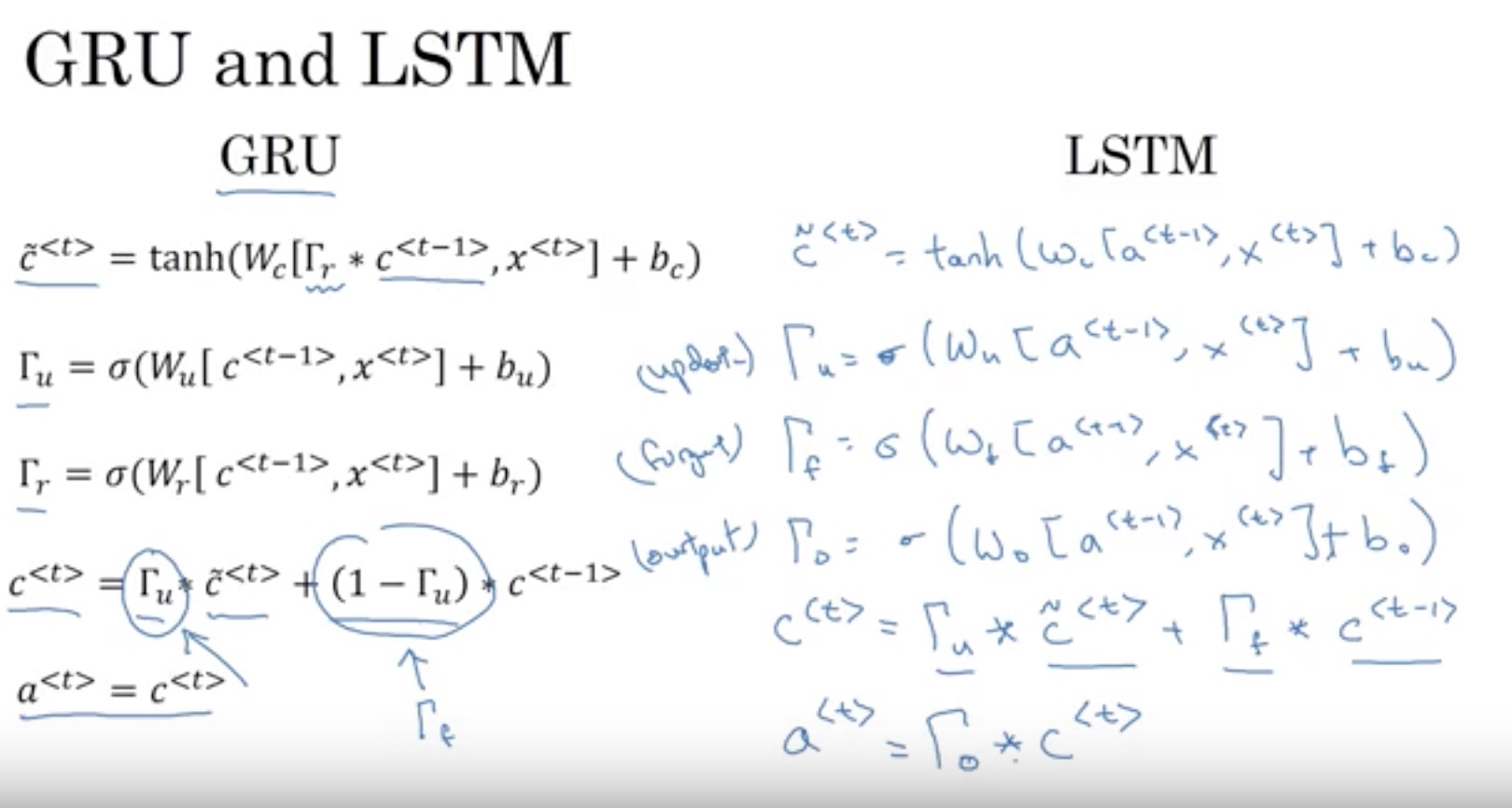
LSTM

The chain rule results in vanishing, thus, if we change this structue into combination of sum terms.

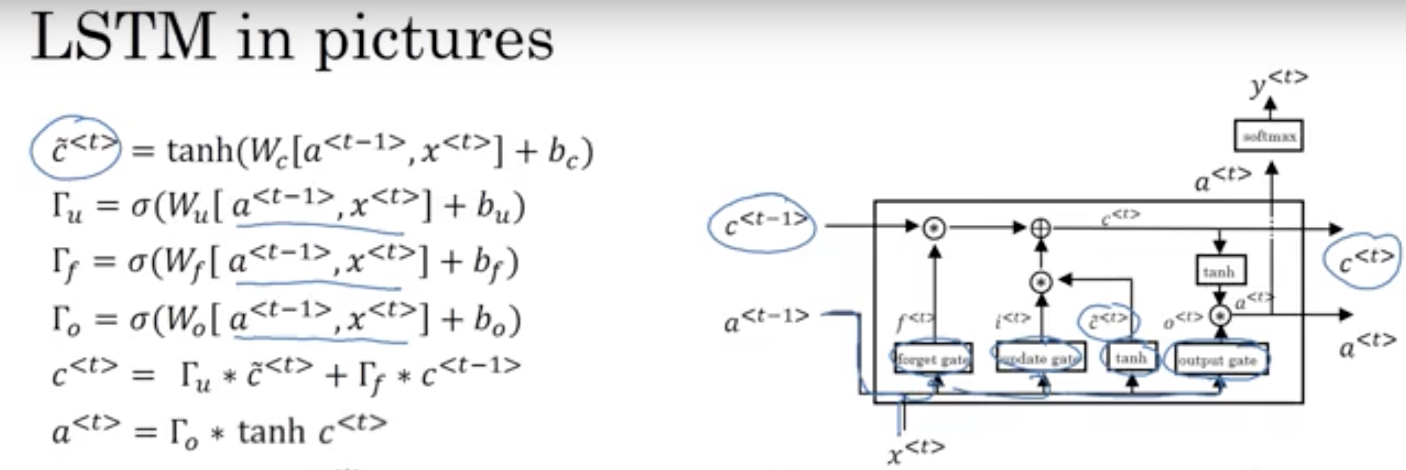
The cell state in LSTM is linear combination of current state and previous state, which avoid the gradient vanishing.

GRU

The GRU simplifies the output and remove forget gate in LSTM.