介绍
这个是hugo的deep learning的学习tutorial,需要慢慢刷掉,当然cmu 10707 的slides很多也是参考这个的(Russlan自己说)整理的,你如果找不到CMU 10707的视频你可以看这个,也是极好的。
然后,这里我想整理下最最基本的neural network的公式的推导,自己再推一遍,感觉就不虚:
网络的基本结构:
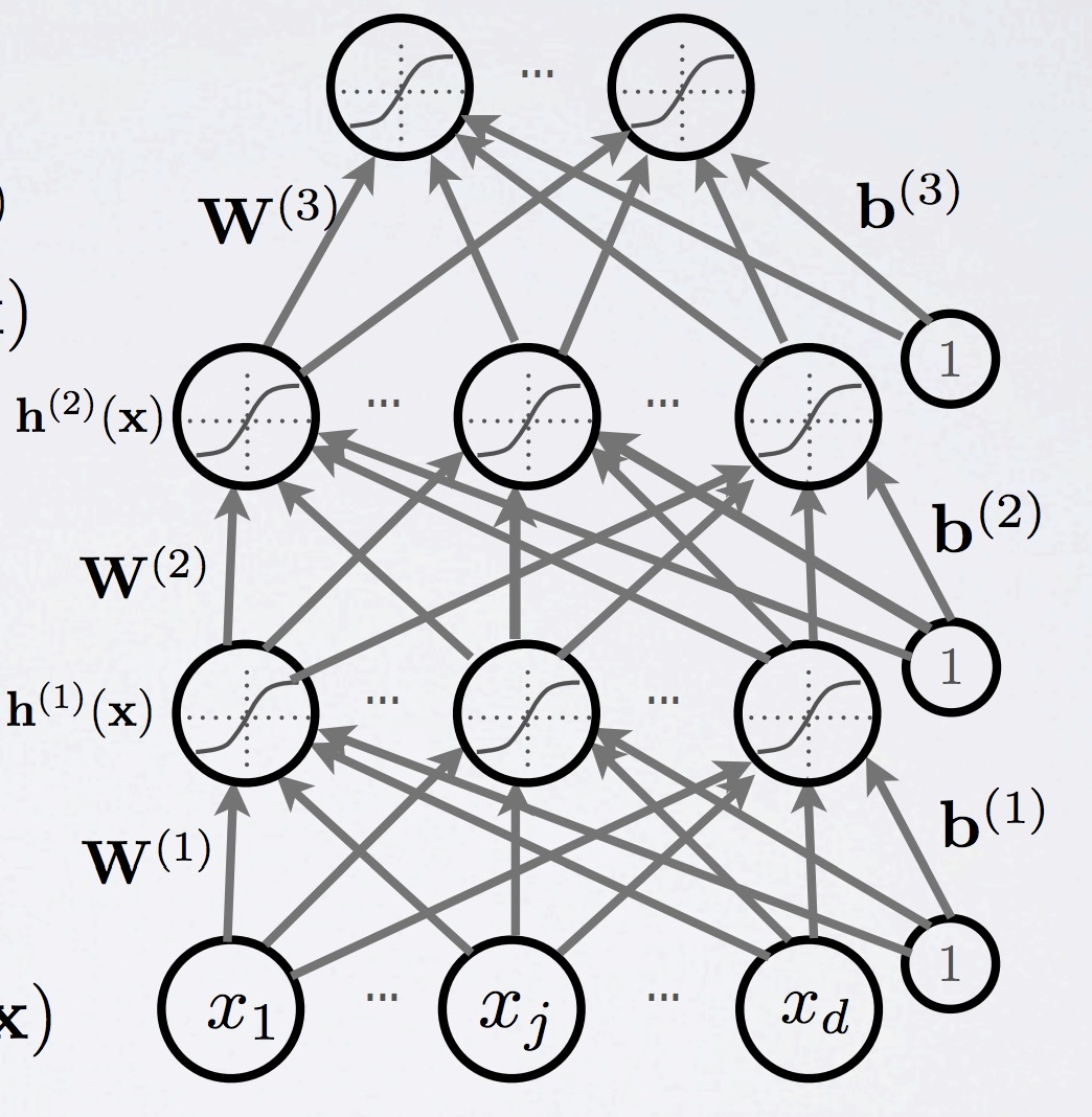
- layer pre-activation for $k > 0$ $(h_{0}(x) = x)$
$a^{(k)}(x) = b^{(k)} + W^{(k)}h^{(k - 1)}(x)$
感觉这么记忆,不会记乱,k就是第几层neuron,然后$h^{(k - 1)}(x)$是前一层的输出,然后weights $W^{(k)}$,bias $b^{(k)}$都是这层的,虽然有前一层输出作为的输入,但是这些还是算这一层的。 hidden layer activation (k from 1 to L)
$h^{(k)}(x) = g(a^{(k)}(x))$
反正这个就是这一层的输出,然后,这层的weights,bias最终都会由这层的输出所终结。output layer activation $k = L + 1$:
$h^{(L + 1)}(x) = o(a^{(L + 1)}(x)) = f(x)$
和hidden不一样就是这个是最后一层了,然后这层的activation function也会和之前hidden layers有所不同,如果是分类的话,往往是softmaxsoftmax activation function at the output:
$o(a) = softmax(a) = [\frac{exp(a_1)}{\sum_c exp(a_c)}…\frac{a_C}{\sum_c exp(a_c)}]^T$
如何理解softmax呢,为什么多分类问题里面要用softmax呢,而不是别的呢?
知乎对此有一定的讨论,我这里引用下王赟(yun第一声)大神的解答:- 原因之一:希望特征对概率的影响是乘性的
- 原因之二:多类分类问题的目标函数常常选为cross-entropy,…(推完整个,回来补)
activation function:
sigmoid:
- formula:
$\sigma(x) = \frac{1}{1 + e^{-x}}$,$\sigma(x)’ = \frac{e^x}{(1 + e^x)^2} = (1 - \sigma(x)) \sigma(x)$ - shortcomings:
- gradient vanish
- symmetric
- time cosuming to compute exp
- formula:
tanh:
- formula:
$tanh(x) = \frac{e^x - e^{-x}}{e^x + e^{-x}} = \frac{2}{1 + e^{-2}} - 1 = 2 \sigma(2x) - 1$,$tanh(x)’ = \frac{e^x - e^{-x}}{e^x + e^{-x}}$ - 感觉就是解决了原点对称的问题
- formula:
relu:
- formula:$f(x) = max(0, x)$
- 优点:
Relu会使一部分神经元的输出为0,这样就造成了网络的稀疏性,并且减少了参数的相互依存关系,缓解了过拟合问题的发生
计算量小 - 缺点:
部分neuro会死亡
leaky relu:
- formula:$f(x) = max(\epsilon x, x)$
- 优点:
解决了neuron会死亡的问题
maxout:
- formula: 对 relu 和 leaky relu的一般归纳:$f(x) = max(w_1^T x + b_1, w_2^T x + b_2)$
- 优点:
计算简单,不会死亡,不会饱和
loss function:
stochastic gradient descent (SGD):
随机梯度下降应该是最最基础的梯度下降的方法了,- initialize $\theta$ ($\theta = {W^{(1)}, b^{(1)}…,W^{(L + 1)}}$)
- algorithm:
for N iterations: (One epoch)for each training example $(x_{(t)}, y_{(t)})$ $\delta = -\nabla_{\theta}l(f(x_{(t)}, \theta), \y_{(t)}) - \lambda\nabla_{(\theta)}$ $\omiga_{(\theta)}$ $\theta \leftarrow \theta + \alpha \delta$ - SGD 的优缺点:
- 缺点:
- 选择合适的learning rate比较困难 - 对所有的参数更新使用同样的learning rate。对于稀疏数据或者特征,有时我们可能想更新快一些对于不经常出现的特征,对于常出现的特征更新慢一些,这时候SGD就不太能满足要求了
- 相对BGD noise会比较大
- 缺点:
batch gradient descent (BGD) 的对比:
所谓batch就是一起算,你看公式就知道:
$\theta \leftarrow \theta + \frac{1}{m}\sum_{i}(y_i - f(x;\theta)(x_i))$ (MSE)- 缺点:m很大的时候,train的会比较慢
- 优点:比SGD稳定
mini-batch GD:
就是这两个的折中,就像强化学习里面的,TD,Monta Carlo之间的n step-TD- advantages:
- give a accurate estimate of average loss
- can leverage matrix operations, which cost less than BGD
- advantages:
what neural network estimates?
$f(x)_{c} = P(y=c|x)$, where c means which class.what to optimize?
maximize log likelihood —- minize negative log likelihood: $P(y_i=c|x_i)$,given $(x_i, y_i)$
cross-entropy: p, q (p one-hot, q distribution of the P(y=c|x))
$l(f(x), y) = -\sum_c1(y=c)log f(x)_c = - log f(x)_y$
loss gradient output:
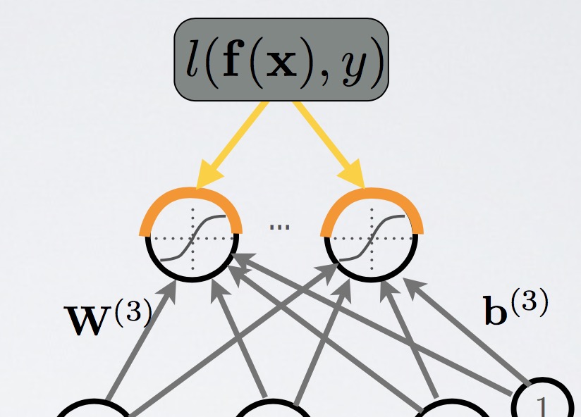
loss gradient at output
partial derivative:
$\frac{\partial - logf(x)_y}{\partial f(x)_c} = \frac{-1^{(y = c)}}{f(x)^y}$
这里,y要和c一样才有值,因为这里cross-entropy里面用了one-hot,只有在同一维度下面,求偏导才有值。gradient:
然后,我们推广到,求梯度
$\nabla_{f(x)} -logf(x)_y= \frac{-1}{f(x)_y} [1^{(y=0)}…1^{(y=C-1)}]^T = \frac{-e(y)}{f(x)^y}$
loss gradient at output pre-activation
partial derivative:
首先还是标量的形式,
$\frac{\partial - logf(x)_y}{\partial a^{(L+1)}(x)_c} = (1^{(y = c)}} - f(x)^y)$
这里,y要和c一样才有值,因为这里cross-entropy里面用了one-hot,只有在同一维度下面,求偏导才有值。gradient:
然后,我们类比到向量上面,
$\nabla_{a^{(L+1)}(x)_c}[- logf(x)_y}] = -(e^{(y)}} - f(x)^y)$proof:
这里的proof不完整,只是推了一个维度的,完整的可以参考ece一个师兄的知乎的矩阵求导术,之后回来在补推一下。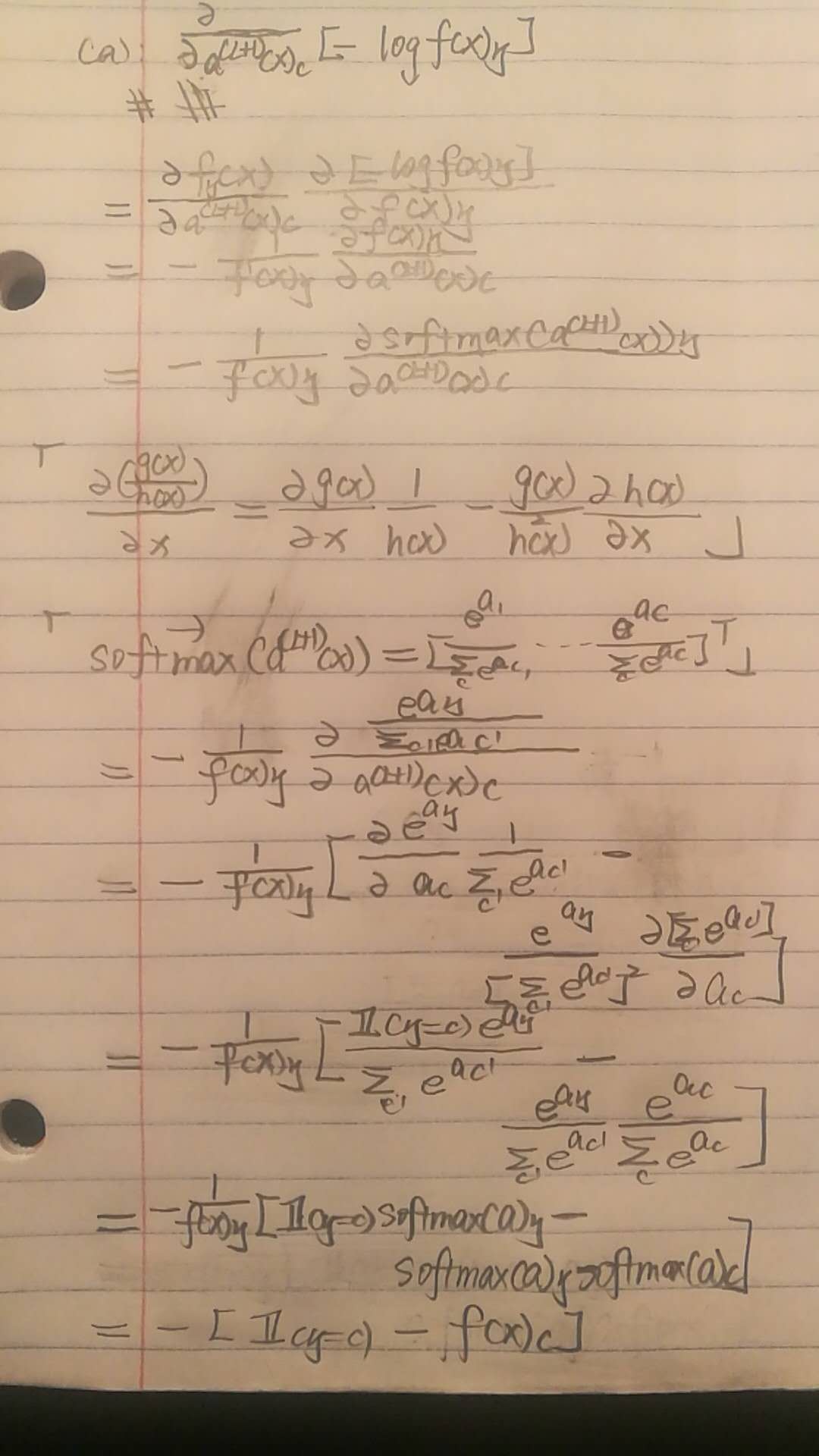
Backpropagation
Compute output gradient (before activation)
$\nabla_{a^{(L+1)}(x)} -logf(x)_y \leftarrow - (e(y)-f(x))$
for k from L + 1 to 1
- compute gradients of hidden layer parameter
$\nabla_{W^{(k)}} -logf(x)^y \leftarrow $ $\nabla_{a^{(k)}(x)} -log f(x)^y h^{(k-1)}(x)^T$
$\nabla_{b^{(k)}} -logf(x)^y \leftarrow $ $\nabla_{a^{(k)}(x)} -log f(x)^y$ - compute gradient of hidden layer below
$\nabla_{b^{(k)}} -logf(x)^y \leftarrow $ $\nabla_{a^{(k)}(x)} -log f(x)^y$ - compute gradient of hidden layer below
$\nabla_{h^{(k-1)}(x)} -logf(x)^y \leftarrow $ $W^{(k)T} \nabla_{a^{(k)}(x)} -log f(x)^y$ - compute gradient of hidden layer below (before activation)
$\nabla_{a^{(k-1)}(x)} -logf(x)^y \leftarrow $ $(\nabla_{h^{(k-1)}(x)} -log f(x)^y) \odot […,g’(a^{(k-1)}(x)_j),…]$
Regularization
L1 & L2 regularization
- L1 $\frac{\lambda}{2m} \sum |w|^2$
L2 regularization is also known as weight decay as it forces the weights to decay towards zero (but not exactly zero). - L2 $\frac{\lambda}{2m} \sum |w|$
Unlike L2, the weights may be reduced to zero here. Hence, it is very useful when we are trying to compress our model. Otherwise, we usually prefer L2 over it. Sparse solution.
- L1 $\frac{\lambda}{2m} \sum |w|^2$
Dropout
So what does dropout do? At every iteration, it randomly selects some nodes and removes them along with all of their incoming and outgoing connections as shown below.
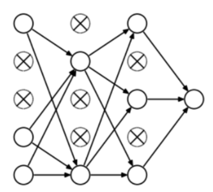
So each iteration has a different set of nodes and this results in a different set of outputs. It can also be thought of as an ensemble technique in machine learning.Ensemble models usually perform better than a single model as they capture more randomness. Similarly, dropout also performs better than a normal neural network model.
This probability of choosing how many nodes should be dropped is the hyperparameter of the dropout function. As seen in the image above, dropout can be applied to both the hidden layers as well as the input layers.
Batch Normalization
- idea
is that since it’s benefit to training if the input data is normalized, so why not normalize in hidden layers to solve the internal covariance shift. - denormalization
to avoid extra effect of normalization, the denormalization parameters are helpful to adjust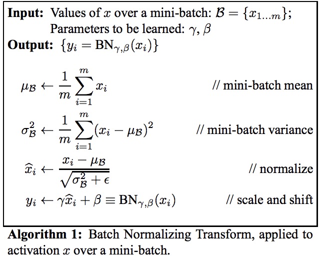
- idea